Transfer Learning

If you want to try transfer learning based approaches on Biquality Data, it is recommended to used dedicated library for Domain Adaptation and Transfer Learning such as ADAPT.

Inductive Transfer Learning

Transfer learning aims to leverage the knowledge gained from solving one task to solve another task, because the first task is deemed useful to solve the latter more efficiently.

Inductive Transfer Learning is the closest sub-field of Transfer Learning to Biquality Learning. For a source and a target task \(U\) and \(V\), it follows the following assumptions on the training data:

• Same input domain: \(\mathcal{X}_T=\mathcal{X}_U\)

• Same output domain: \(\mathcal{Y}_T=\mathcal{Y}_U\)

• No covariate shift: \(\mathbb{P}_T(X)=\mathbb{P}_U(X)\)

• Different conditional distribution: \(\mathbb{P}_T(Y|X)\neq\mathbb{P}_U(Y|X)\)

However, as it is assumed that the source task is deemed useful to solve the target task, transfer learning based approaches are not fit for highly untrustable datasets.

TrAdaBoostClassifier is an algorithm that reuses ideas from the original AdaBoost algorithm [FS1995] to construct a novel transfer learning approach [DYXY2008].

• For the trusted dataset, TrAdaBoost focus on misclassified examples by assigning them higher weights as these examples are considered more difficult and better for generalization [ZZRH2009].

• For the untrusted dataset, however, misclassified examples are deemed useless for the trusted task and thus see their weights decrease following the Weighted Majority Algorithm [LW1994].

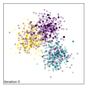
Evolution of sample weights on a toy dataset corrupted with background noise.

Moreover, TrAdaBoostClassifier implements the weight drift correction [ASC2011] but has been extended to take into account a learning rate and multiclass classification with the SAMME algorithm.

References:

[FS1995]

25. Freund, and R. Schapire, “A Decision-Theoretic Generalization of On-Line Learning and an Application to Boosting”, 1997.

[ZZRH2009]

10. Zhu, H. Zou, S. Rosset, T. Hastie. “Multi-class AdaBoost”, 2009.

[DYXY2008]

Wenyuan Dai, Qiang Yang, Gui-Rong Xue, Yong Yu. “Boosting for Transfer Learning”, 2007.

[LW1994]

14. Littlestone, M.K. Warmuth, “The Weighted Majority Algorithm”, 1994.

[ASC2011]

Al-Stouhi, Samir, and Chandan K. Reddy. “Adaptive Boosting for Transfer Learning Using Dynamic Updates”, ECML/PKDD 2011.

Supervised Domain Adaptation

Domain adaptation refers to the process of adapting a model trained on one distribution of data to work well on a different distribution of data. This is often necessary because it is impractical or impossible to collect a large enough dataset to train a model that can generalize well for all possible inputs it may encounter in practice.

Supervised Domain Adaptation is the closest sub-field of Domain Adaptation to Biquality Learning. For a source and a target task \(U\) and \(V\), it follows the following assumptions on the training data:

• Same input domain: \(\mathcal{X}_T=\mathcal{X}_U\)

• Same output domain: \(\mathcal{Y}_T=\mathcal{Y}_U\)

• Covariate shift: \(\mathbb{P}_T(X)\neq\mathbb{P}_U(X)\)

• Same conditional distribution: \(\mathbb{P}_T(Y|X)=\mathbb{P}_U(Y|X)\)

As such Supervised Domain Adaptation algorithms are not able to handle changes or perturbation in the decision boundary but can still be interesting approaches as baselines.

EasyADAPT [H2007] is one of these Supervised Domain Adaptation algorithms that creates an augmented input space \(\tilde{\mathcal{X}} = \mathcal{X}^3\) with two different mapping for untrusted (or source) and trusted (or target) samples, \(\Phi_U:\mathcal{X}\mapsto \tilde{\mathcal{X}}\) and \(\Phi_T:\mathcal{X}\mapsto \tilde{\mathcal{X}}\).

• \(\forall \mathbf{x} \in \mathcal{X}, \Phi_U(\mathbf{x})=<\mathbf{x}, \mathbf{x}, \mathbf{0}>\)

• \(\forall \mathbf{x} \in \mathcal{X}, \Phi_T(\mathbf{x})=<\mathbf{x}, \mathbf{0}, \mathbf{x}>\)

This augmented domain \(\tilde{\mathcal{X}}\) allow for the classifier to learn different relation between the features and the target differently for the untrusted, trusted and general domain.

For example, when using the (upscaled) digits dataset as a source dataset to learn USPS classification, the augmented image would be composed of three images, one blank and the input image repeated twice.

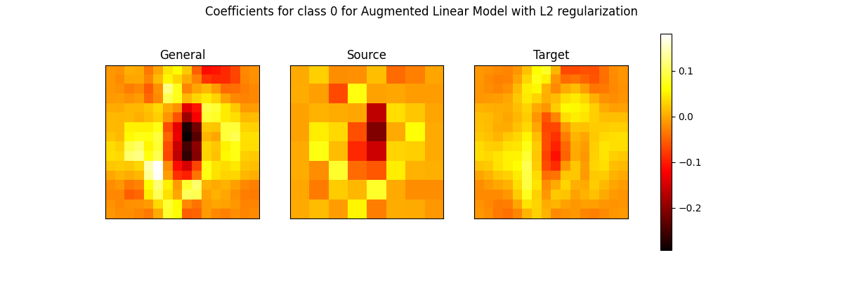
The augmented dataset allows the model to learn distinct features for source and target images, but also general features common between the two datasets.

References:

[H2007]

Daumé III, Hal. “Frustratingly Easy Domain Adaptation.” Proceedings of the 45th Annual Meeting of the Association of Computational Linguistics. 2007.

K-Domain Adaptation

However, when looking at the distribution of features in Biquality Data given a class \(\mathbb{P}(X|Y=y)\), we can observe a change in distribution between the two datasets.

Indeed, given the Bayes Formula \(\mathbb{P}(X|Y) = \frac{\mathbb{P}(Y|X)\mathbb{P}(X)}{\mathbb{P}(Y)}\), and at \(\mathbb{P}(X)\) and \(\mathbb{P}(Y)\) constant, corrupting \(\mathbb{P}(Y|X)\) is equivalent to corrupting \(\mathbb{P}(X|Y)\).

We illustrate this behavior with the following toy dataset where untrusted samples have been corrupted with Completly at Random label noise:

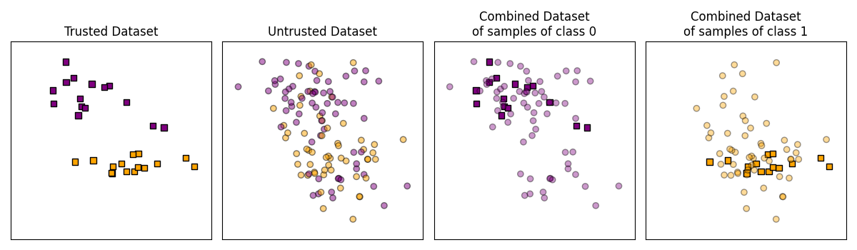
Illustration of the equivalence of Conditional Covariate Shift and Concept Drift on a toy dataset.

In the previous Figure, we observe that some untrusted samples of class 0 (in purple) seem to be out of the normal distribution for trusted samples of class 0 (in red). The same behavior can be observed for samples of class 1 (respectively in green and blue).

Thanks to these observations, one approach to designing Biquality Learning algorithms is to use one Unsupervised Domain Adaptation method per class. This approach is called K-Domain Adaptation (with K being the number of classes).

One K-Domain Adaptation family of algorithms named K-Density Ratio is implemented in biquality-learn and is documented in Radon-Nikodym Derivative.