Augmented Dataset with Easy Adapt

This example shows how EasyAdapt works on a toy domain adaptation problem from the digits dataset to the USPS dataset.

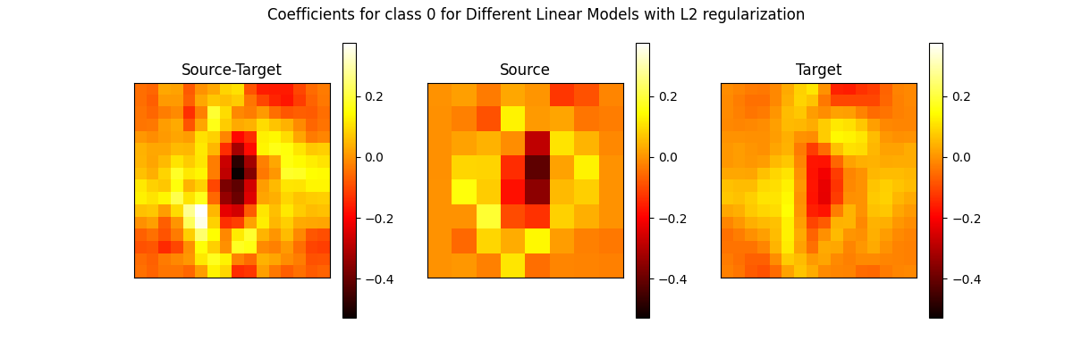
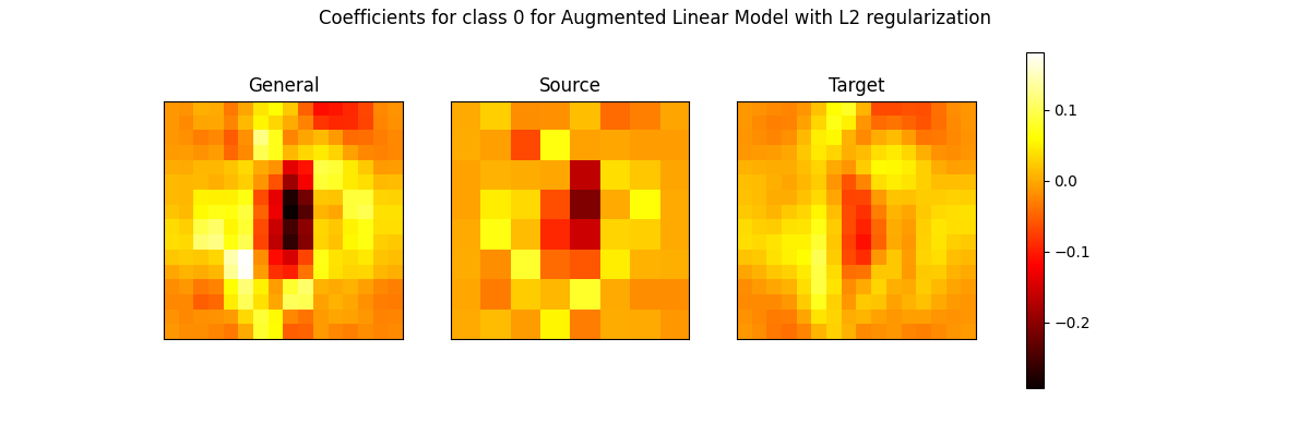
We illustrate the two set of coefficients for the class 0 from different linear models learned from source and target dataset or from the augmented dataset.

import matplotlib.pyplot as plt
import numpy as np
from sklearn.base import clone
from sklearn.datasets import fetch_openml, load_digits
from sklearn.linear_model import LogisticRegression
from sklearn.model_selection import train_test_split
from sklearn.pipeline import make_pipeline
from sklearn.preprocessing import LabelEncoder, StandardScaler

from bqlearn.ea import EasyADAPT

seed = 42

X_digits, y_digits = load_digits(return_X_y=True)
X_usps, y_usps = fetch_openml(data_id=41070, return_X_y=True, as_frame=False)

# ??
y_usps = y_usps - 1

# Rescale the digits dataset
X_digits = X_digits.reshape(-1, 8, 8)
X_digits = np.repeat(X_digits, 2, axis=1)
X_digits = np.repeat(X_digits, 2, axis=2)
X_digits = X_digits.reshape(-1, 16 * 16)

# Split the target dataset
X_usps, X_test, y_usps, y_test = train_test_split(
    X_usps, y_usps, train_size=100, stratify=y_usps, random_state=seed
)

# Rescale
scale_usps = StandardScaler().fit(X_usps)
X_usps = scale_usps.transform(X_usps)
X_test = scale_usps.transform(X_test)
X_digits = StandardScaler().fit_transform(X_digits)

# Prepare Data
X = np.vstack((X_digits, X_usps))
y = np.hstack((y_digits, y_usps))
sample_quality = np.hstack((np.zeros(X_digits.shape[0]), np.ones(X_usps.shape[0])))

encoder = LabelEncoder().fit(y)
y = encoder.transform(y)
y_test = encoder.transform(y_test)

# Base Classifier
clf = LogisticRegression(max_iter=int(1e6))

/home/docs/checkouts/readthedocs.org/user_builds/biquality-learn/envs/latest/lib/python3.10/site-packages/sklearn/datasets/_openml.py:971: UserWarning: Version 1 of dataset USPS is inactive, meaning that issues have been found in the dataset. Try using a newer version from this URL: https://api.openml.org/data/v1/download/18805612/USPS.arff
  warn(
/home/docs/checkouts/readthedocs.org/user_builds/biquality-learn/envs/latest/lib/python3.10/site-packages/sklearn/datasets/_openml.py:1002: FutureWarning: The default value of `parser` will change from `'liac-arff'` to `'auto'` in 1.4. You can set `parser='auto'` to silence this warning. Therefore, an `ImportError` will be raised from 1.4 if the dataset is dense and pandas is not installed. Note that the pandas parser may return different data types. See the Notes Section in fetch_openml's API doc for details.
  warn(

st = clone(clf).fit(X, y)
s = clone(clf).fit(X_digits, y_digits)
t = clone(clf).fit(X_usps, y_usps)

ea = make_pipeline(EasyADAPT(), clf)
ea.fit(X, y, easyadapt__sample_quality=sample_quality)

Pipeline(steps=[('easyadapt', EasyADAPT()),
                ('logisticregression', LogisticRegression(max_iter=1000000))])

In a Jupyter environment, please rerun this cell to show the HTML representation or trust the notebook.
On GitHub, the HTML representation is unable to render, please try loading this page with nbviewer.org.

vmin = float("inf")
vmax = float("-inf")

for clf in [st, s, t]:
    small = np.min(clf.coef_[0, :])
    big = np.max(clf.coef_[0, :])
    if small < vmin:
        vmin = small
    if big > vmax:
        vmax = big

clfs = [st, s, t]
names = ["Source-Target", "Source", "Target"]

fig, axs = plt.subplots(1, 3, figsize=(12, 4))
for i, clf in enumerate(clfs):
    ax = axs[i]
    imp_reshaped = clf.coef_[0, :].reshape(16, 16)
    mat = ax.matshow(imp_reshaped, cmap=plt.cm.hot, vmin=vmin, vmax=vmax)
    fig.colorbar(mat, ax=ax)
    ax.set_title(names[i])
    ax.set_xticks(())
    ax.set_yticks(())

# fig.colorbar(mat, ax=axs)
fig.suptitle(
    "Coefficients for class 0 for Different Linear Models with L2 regularization"
)
plt.show()

importances = np.split(ea[-1].coef_[0, :], 3)
names = ["General", "Source", "Target"]

vmin = np.min(ea[-1].coef_[0, :])
vmax = np.max(ea[-1].coef_[0, :])

fig, axs = plt.subplots(1, 3, figsize=(12, 4))
for i, imp in enumerate(importances):
    ax = axs[i]
    imp_reshaped = imp.reshape(16, 16)
    mat = ax.matshow(imp_reshaped, cmap=plt.cm.hot, vmin=vmin, vmax=vmax)
    ax.set_title(names[i])
    ax.set_xticks(())
    ax.set_yticks(())

fig.colorbar(mat, ax=axs)
fig.suptitle(
    "Coefficients for class 0 for Augmented Linear Model with L2 regularization"
)
plt.show()

print(f"Performance of source-target linear model : {st.score(X_test, y_test)}")
print(f"Performance of source linear model : {s.score(X_test, y_test)}")
print(f"Performance of target linear model : {t.score(X_test, y_test)}")
print(f"Performance of augmented linear model : {ea.score(X_test, y_test)}")

Performance of source-target linear model : 0.8314851054577082
Performance of source linear model : 0.6863448575777343
Performance of target linear model : 0.8430093498586649
Performance of augmented linear model : 0.8499673842139596